The data
Data of some helthcare indicators in Catalonia is publicly available from the Open Data Repository of the Observatori del Sistema de Salut de Catalunya. We have used the dataset corresponding to year 2017 (you can download it here). This is an Excel file providing indicators at three different levels (territorial units) in different tabs. We concentrate on tab Analisi AGA, containing indicators for the so called healthcare management areas (àrees de gestió assistencial, or AGA, in Catalan).
In the following, we assume some familiarity with R, particularly with basic functions of the dplyr package to work with dataframes, and chaining operations with the pipe (%>%) operator.
We first use package readxl to read the data in tab Analisi AGA of the Excel file, select the columns we need and rename them to English, and save the result in a dataframe (aga_data).
library(readxl)
library(dplyr)

read_excel("Taula_resum_territorial_2017.xlsx",
           sheet = "Analisi AGA") %>%
  select(indicator_group = `Àmbit`,
         indicator = Indicador,
         aga_code = `codi AGA`,
         value = `valor AGA total`) -> aga_data
Indicators are grouped in broad topics, recorded in indicator_group. We first look at unique values of this variable to see how many indicator groups there are, and then we list all indicators of a selected group:
# see all groups of indicators
unique(aga_data$indicator_group)
[1] "Dades Generals"
[2] "Atenció primària"
[3] "Salut Mental"
[4] "Prescripció farmacèutica i tractaments"
[5] "Àmbit Hospitalari"
[6] "Àmbit d'Urgències"
[7] "Sociosanitari"
[8] "Llistes d'espera" # see all indicators in a selected group
aga_data %>%
filter(indicator_group == "Prescripció farmacèutica i tractaments") %>%
pull(indicator) %>%
unique()[1] "Població consumidora de fàrmacs pel TDAH de 6 a 17 anys (%)"
[2] "Població consumidora d'IBPs de 50 anys o més (%)"
[3] "Població consumidora de psicofàrmacs de 65 anys o més (%)"
[4] "Població consumidora d'antibiòtics (%)"
[5] "Taxa de població amb polimedicació (10 medicaments o més)"
[6] "Taxa de població amb oxigenoteràpia domiciliària"
[7] "Taxa de població amb CPAP" The map
Maps of the Catalan helthcare territorial structure can be downloaded here. This is a compressed (.zip) file, containing a folder named ABS_2018, which in turn contains several files for different territorial units and file formats. After extracting the contents of the .zip file, we use package sf to read the vector map for AGA’s. We do some renaming, and redefine aga_code so as to be numeric (instead of a factor); this is important, since we will later need this variable as key to merge with the data in aga_data. Finally, we simplify the map to reduce the weight of the resulting object, saved as aga_map.
library(sf)

st_read(dsn = "../R Catalonia maps/ABS_2018/AGA_2018.shp") %>%
  select(aga_name = NOMAGA,
         aga_code = CODIAGA,
         geometry) %>%
  mutate(aga_code = as.numeric(as.character(aga_code))) %>%
  arrange(aga_code) %>%
  st_simplify(dTolerance = 10) -> aga_map
As seen in the next outputs, aga_map is a dataframe containing standard columns (aga_name, aga_code), plus a list column (geometry) containg the geographic information of AGA’s needed to draw the map. Looking carefully at aga_name in the 6th row of the last output, a problem with encoding is detected, because letters with accent are not well written (<e0> instead of à). Since aga_name is a factor, we fix the problem by defining appropriate encoding for its levels, and verify.
class(aga_map)[1] "sf" "data.frame"head(aga_map)Simple feature collection with 6 features and 2 fields
geometry type: GEOMETRY
dimension: XY
bbox: xmin: 275940.3 ymin: 4562093 xmax: 419215.8 ymax: 4747976
epsg (SRID): NA
proj4string: +proj=utm +zone=31 +ellps=GRS80 +units=m +no_defs
aga_name aga_code geometry
1 Alt Urgell 1 MULTIPOLYGON (((377643.2 46...
2 Cerdanya 2 MULTIPOLYGON (((417782.2 46...
3 Pallars 3 POLYGON ((348731.1 4674932,...
4 Aran 4 POLYGON ((320139.5 4720858,...
5 Lleida 5 POLYGON ((319752.2 4581218,...
6 Alt Camp i Conca de Barber<e0> 6 POLYGON ((354980.7 4566136,...class(aga_map$aga_name)[1] "factor"Encoding(levels(aga_map$aga_name)) <- "latin-1"
head(aga_map)Simple feature collection with 6 features and 2 fields
geometry type: GEOMETRY
dimension: XY
bbox: xmin: 275940.3 ymin: 4562093 xmax: 419215.8 ymax: 4747976
epsg (SRID): NA
proj4string: +proj=utm +zone=31 +ellps=GRS80 +units=m +no_defs
aga_name aga_code geometry
1 Alt Urgell 1 MULTIPOLYGON (((377643.2 46...
2 Cerdanya 2 MULTIPOLYGON (((417782.2 46...
3 Pallars 3 POLYGON ((348731.1 4674932,...
4 Aran 4 POLYGON ((320139.5 4720858,...
5 Lleida 5 POLYGON ((319752.2 4581218,...
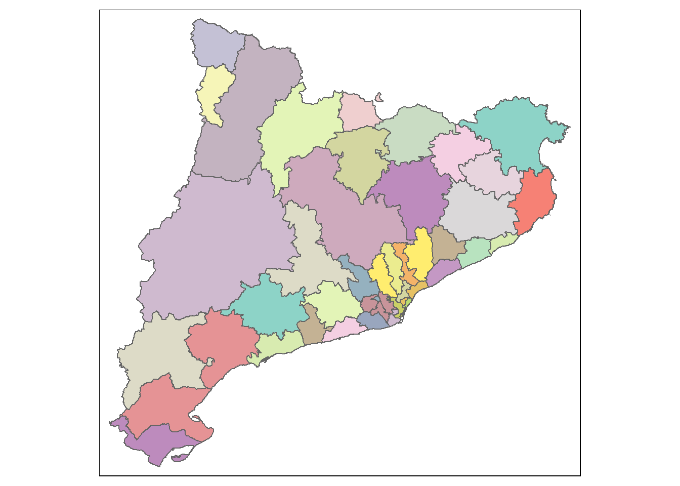
6 Alt Camp i Conca de Barberà 6 POLYGON ((354980.7 4566136,...We can now plot the map of AGA’s using package tmap, with the following code:
library(tmap)

tm_shape(aga_map) +
  tm_polygons("aga_name", legend.show = FALSE)
Showing an indicator in the map
Much more interesting is to show a specific indicator in the map of AGA’s. To achieve this, we first need to subset aga_data for the indicator of interest, and then merge the result to aga_map. Note that the merge is based on variable aga_code, which is common to both dataframes.
aga_data%>%
  filter(indicator == "Població consumidora d'antibiòtics (%)") -> ab_data

# merge map and data
left_join(aga_map, ab_data) -> ab_map
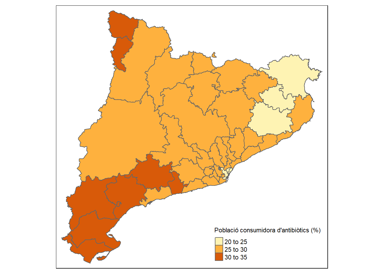
Joining, by = "aga_code"Finally, we plot the value of the selected indicator on the map. We take advantage of the fact that indicator is a constant in ab_map to define the title of the plot as unique(ab_map$indicator).
tm_shape(ab_map) +
  tm_polygons("value", title = unique(ab_map$indicator))
In the previous static map we see that this indicator takes values in the range 20 - 35, and some heterogeneity is apparent among AGA’s. However, it is hard to identify what are the specific AGA’s showing lower values, particularly, small areas in Barelona city. A better option that overcomes this limitation is to produce an interactive map. Happily, this only takes changing the visualization mode, and then executing exactly the same code that produced the static map above, as done in the following code. Note that, on hovering over any AGA, the name of the AGA is shown in a popup and, on clicking, the actual value of the indicator is also shown. In addition, by zooming in we can easily identify three smaller AGA’s in Barcelona city with low values of the indicator: Barcelona Esquerra, Barcelona Dreta, and Barcelona Litoral Mar.
tmap_mode("view")

tm_shape(ab_map) +
  tm_polygons("value", title = unique(ab_map$indicator))
Last, note that the visualization mode will remain unchanged until you explicitly redefine it with tmap_mode("plot"), or ttm() (which toggles between the two modes).
More indicators
The following function allows to produce similar plots for other indicators, with little effort. The call of the function providing the desired indicator as argument, will produce the plot. Optionally, a second argument can be provided for the legend title.
# define the function
get_indicator_map <- function (ind, ind_title = ind) {

  aga_map %>%
    left_join(filter(aga_data, indicator == ind)) %>%
    tm_shape() +
    tm_polygons("value",
                title = ind_title)

}

# call the function
get_indicator_map("Taxa de població amb polimedicació (10 medicaments o més)",
                  "Població polimedicada")
For more on maps and how to plot them with R, see Geocomputation with R.